
Below you will find movies of phase-field simulations of multiphase and multicomponent systems from my PhD thesis, and a paper that I published in Physical Review E.

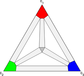
I studied microstructure formation in ternary systems and developed simulations for the phase diagrams pictured to the right. The diffusing components are colored red, green and blue, and there are three solid phases: a red-rich phase, a green-rich phase, and a blue-rich phase. A silver liquid phase appears in the center of the triangle, and it’s appearance is controlled by a dimensionless temperature.
I developed new way of visualizing ternary phase-field simulations by rendering movies with two different panes. In the left pane, a ternary triangle is drawn, and in the right pane an images of the ternary microstructure is drawn with the three components colored red, green, and blue. The phases, which are red-rich, blue-rich, and green-rich, in the examples presented here, and thus phase can be inferred from the composition picture. The second pane shows an RGB image of the microstructure with the liquid phase colored light gray.
For every composition in the evolving microstructure, a corresponding point is drawn on the ternary triangle at the appropriate composition. The color of the point matches the color of the composition in the microstructure. The ternary triangle frame gives insight into which compositions are present in the microstructure, and the motion of the points reveals the path the system takes to reach equilibrium. By comparing the ternary composition triangle to the phase diagram, it becomes clear which phases are present in the microstructure, and, with knowledge of the mean microstructure composition, which of the phases are stable and which are metastable.
Rings
This video shows growth of a critical nuclei of reddish solid from a liquid of composition 35% red, 31% green, 34% blue (located near the center of the ternary triangle). Solidification proceeds by producing alternating rings of the red rich, blue rich, and green rich phases. The composition triangle is particularly fascinating to watch. As each new phase nucleates, it produces a loop in composition space. The loop disappears at later times as the interface approaches equilibrium. The loop is a result of the Gibbs-Thomson effect and the fact that curvature of the inner and outer interface of each ring differ.
Kaleidoscopic microstructure
This video on the right shows the growth of kaleidoscopic microstructure that grows from a critical nucleus placed in a ternary eutectic liquid. The changing radius of curvature of the growing particle disrupts the formation of lamellar structures resulting in complex random patterns. The symmetry is likely a result of the symmetry of the initial nucleus, the square grid, and the periodic boundaries. Small changes in the size and shape of the initial nucleus, the interfacial energy between different phases, and mobilities produce completely different random patterns.
Nucleation and formation of intergranular films
This video shows nucleation in a four phase ternary system. The system is initially a metastable liquid phase with composition 35% red, 31% green, 34% blue. The temperature in this model is low enough that there is no stable liquid region, although there is a region in the center of the phase diagram where the free energy curve for the liquid is lower than all of the solid curves. Liquid in this region is metastable, and noise must be added to overcome an energy barrier and nucleate solid. The nucleation procedure developed in this work was used. As nuclei grow, spinodal decomposition appears to occur in front of the advancing interfaces.Halfway through the simulation the temperature is increased. There is still no stable liquid region at this higher temperature, but stable intergranular liquid films are observed to form first at triple junctions and later at grain boundaries. The composition triangle shows how, when the temperature is increased, the composition at the interfaces is attracted toward the center of the triangle where the metastable portion liquid free energy curve is located. Small grains are observed to dissolve back into the liquid while large grains consume liquid.
Here is exactly the same simulation except that diffusivity of the components in the solid has been slowed to 1/1000th of their diffusivity in the liquid. The composition triangle shows that a metastable microstructure forms. The composition of each grain is not its equilibrium composition. When the temperature is increased, a larger area of the microstructure melts, and the grains slowly approach their equilibrium compositions.
Cellular solidification
An interesting recent discovery is that a cellular solidification morphology improves the mechanical performance of transient liquid bonds compared to bonds with a flat bond interface while decreasing bonding time. Planar solidification was disrupted by performing transient liquid bonding with a temperature gradient across the interface, which induces a composition gradient in the liquid. It is thought that a planar bond line tends to concentrate oxides and other impurities and does not provide as much bonding surface area as a wavy bond line. Being able to control the morphology very carefully is important because the formation of dendrites was found to weaken the bond.
A simulation of a cellular structure during the isothermal solidification stage of a transient liquid bond is shown to the right, with the liquid phase colored silver. In order to trigger cellular growth, several phase-field parameters were adjusted from the previous simulation. First, the composition of the liquid was moved closer to the red-rich phase: c=(.7,.15,.15). This would be achieved experimentally by performing the TLPB dissolution stage at a higher temperature than in the original simulation so that the liquid phase region would be larger. Second, the liquid was made unstable by quenching the system to a temperature of T=-.2. Third, the diffusivity of the components in the solid was set to 1/1000 the diffusivity in the liquid to more closely agree with experimental observations. Finally, the phase barrier height was increased, and the velocity of the solidifying interface was increased by decreasing the relaxation parameter.
Transient liquid bonding
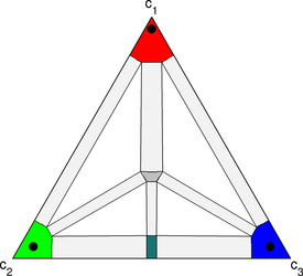
This video demonstrates transient liquid bonding using 5-phase version of the multiphase model being developed. The corresponding phase diagram is shown to the right. A stable compound of 50% green, 50% blue has been added to the free energy landscape, and the temperature is held at a value where there is a small region of stable liquid (located at the center of the phase diagram). In the simulation, a thin strip of the compound is placed between two blocks of the reddish phase. The volume fraction of compound is small and does not significantly change the mean composition of the system – even with the strip of compound, the system remains in the single reddish phase region of the phase diagram. As the simulation progresses, the strip begins to dissolve and liquid is observed to form at the interfaces between the strip and the red phase. The liquid grows inward toward the center of the strip as red diffuses in, and liquid eventually consumes the strip. As time progresses further, the liquid disappears as the green and blue components diffuse out of the liquid and into the red phase where they exist in low concentrations at equilibrium.
Reactive liquid bonding
This simulation is similar to the one above, except that rather than starting with a thin strip of the green-blue compound, thin strips of green-rich and blue-rich phases are put at the junction. What results is a reaction between the green and blue to form the compound, followed by the formation of a transient liquid which then joins the two pieces of red.